Multiple Regression using Python

Table of Contents

Whenever I do any machine learning I either manually implement models in MATLAB or use Python libraries like scikit-learn where all of the work is done for me. However, I wanted to learn how to manually implement some of these things in Python so I figured I’d document this learning process over a series of posts. Lets start with something simple: ordinary least squares multiple regression.

The goal of multiple regression is predict the value of some outcome from a series of input variables. Here, I’ll be using the Los Angeles Heart Data

Setting up the data

Let's import some modules:

import numpy as np
import matplotlib.pyplot as plt

Next, we’ll need to load the dataset:

dataset = np.genfromtxt('regression_heart.csv', delimiter=",")

We’ll need to create a design matrix (x) containing our predictor variables, and a vector (y) for the outcome we’re trying to predict. In this case, I’m just going to predict the first column from all of the others for demonstration purposes.

We can use slicing to grab every row and all columns (after the first) to create x.

x = dataset[:, 1:]

Optionally, we can scale (standardize) the data so gradient descent has an easier time converging later:

x = (x - np.mean(x, axis=0)) / np.std(x, axis=0)

We’ll need to add a column of 1’s so we can estimate a bias/intercept:

x = np.insert(x, 0, 1, axis=1) # Add 1's for bias

We can do the same thing to pull out the first column to create y. We want this as a column vector for later so we need to reshape it:

y = dataset[:, 0]
y = np.reshape(y, (y.shape[0], 1))

Training the model

First we need to initialize some weights. We should also initialize some other variables/parameters that we’ll use during training:

alpha = 0.01 # Learning rate
iterations = 1000 # Number of iterations to train over
 
theta = np.ones((x.shape[1], 1)) # Initial weights set to 1
m = y.shape[0] # Number of training examples. Equivalent to x.shape[0]
cost_history = np.zeros(iterations) # Initialize cost history values

At this stage, our weights (theta) will just be set to some initial values (1’s in this case) that will be updated during training:

array([[ 1.],
       [ 1.],
       [ 1.],
       [ 1.],
       [ 1.],
       [ 1.],
       [ 1.],
       [ 1.],
       [ 1.],
       [ 1.],
       [ 1.],
       [ 1.],
       [ 1.],
       [ 1.],
       [ 1.],
       [ 1.],
       [ 1.]])

The actual training process for multiple regression is pretty straightforward.

For a given set of weight values, we need to calculate the associated cost/loss:

1. Evaluate the hypothesis by multiplying each variable by their weight
2. Calculate the residual and squared error
3. Calculate the cost using quadratic loss

h = np.dot(x, theta)
residuals = h - y
squared_error = np.dot(residuals.T, residuals)
cost = 1.0/(2*m) * squared_error # Quadratic loss

Now that we know how ‘wrong’ our current set of weights are, we need to go back and update those weights to better values. ‘Better’ in this case just means weight values that will lead to a smaller amount of error. We can use (batch) gradient descent to do this.

I won’t go into details about gradient descent here. The general idea is that we are trying to minimize the cost and to do that we can calculate the partial derivative (gradient) with respect to the weights. Once we know the gradient, we can adjust the value of the weights (theta) in the direction of the minimum. Over many iterations, the weights will converge towards values that will give us the smallest cost value.

Note: the speed of this update is controlled by the learning rate alpha. Setting this value too large can cause gradient descent to diverge, which is not what we want.

gradient = 1.0/m * np.dot(residuals.T, x).T # Calculate derivative
theta -= (alpha * gradient) # Update weights
 
cost_history[i] = cost # Store the cost for this iteration

We simply repeat this entire process over many iterations, and we should end up learning weights that give us the smallest error:

for i in xrange(iterations): # Batch gradient descent
    h = np.dot(x, theta)
    residuals = h - y
    squared_error = np.dot(residuals.T, residuals)
    cost = 1.0/(2*m) * squared_error # Quadratic loss
 
    gradient = 1.0/m * np.dot(residuals.T, x).T # Calculate derivative
    theta -= (alpha * gradient) # Update weights
 
    cost_history[i] = cost # Store the cost for this iteration
 
    if (i+1) % 100 == 0:
        print "Iteration: %d | Cost: %f" % (i+1, cost)

You can see the cost dropping across each iteration:

Iteration: 100  | Cost: 177.951582
Iteration: 200  | Cost: 55.546768
Iteration: 300  | Cost: 38.582054
Iteration: 400  | Cost: 36.015047
Iteration: 500  | Cost: 35.516054
Iteration: 600  | Cost: 35.364456
Iteration: 700  | Cost: 35.296070
Iteration: 800  | Cost: 35.258532
Iteration: 900  | Cost: 35.236041
Iteration: 1000 | Cost: 35.221815

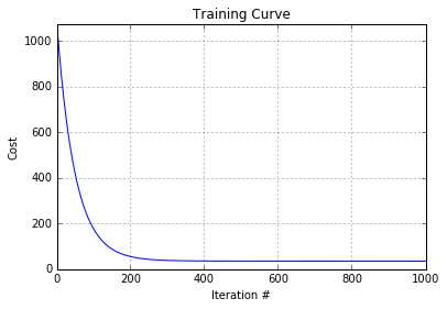
We can visualize learning with a plot. This can be useful for determining whether gradient descent is converging or diverging:

plt.plot(range(1, len(cost_history)+1), cost_history)
plt.grid(True)
plt.xlim(1, len(cost_history))
plt.ylim(0, max(cost_history))
plt.title("Training Curve")
plt.xlabel("Iteration #")
plt.ylabel("Cost")

Visualization

We can visualize learning with a plot. This can be useful for determining whether gradient descent is converging or diverging:

plt.plot(range(1, len(cost_history)+1), cost_history)
plt.grid(True)
plt.xlim(1, len(cost_history))
plt.ylim(0, max(cost_history))
plt.title("Training Curve")
plt.xlabel("Iteration #")
plt.ylabel("Cost")

theta now contains the learned weight values for each variable (including the bias/intercept):

array([[ 46.06305449],
       [  1.0213985 ],
       [  2.35116093],
       [ -0.48043933],
       [ -0.51614245],
       [  1.71466022],
       [  0.95959334],
       [ -0.5916098 ],
       [  1.10940082],
       [  0.68334108],
       [  4.57416498],
       [ -3.38696989],
       [ -0.96933318],
       [ -1.85941235],
       [ -0.14792604],
       [  1.73684471],
       [  1.37675869]])

The full code can be found in my GitHub repo here.