Color image classification (CIFAR-10) using a CNN
Using a convolution neural network to classify images from the CIFAR-10 database
April 4, 2018
Table of Contents
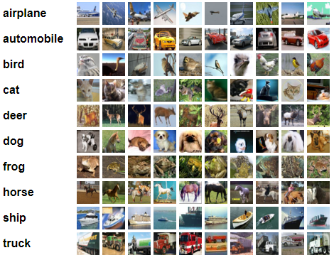
As I mentioned in a previous post, a convolutional neural network (CNN) can be used to classify color images in much the same way as grey scale classification. The way to achieve this is by utilizing the depth dimension of our input tensors and kernels. In this example I’ll be using the CIFAR-10 dataset, which consists of 32×32 color images belonging to 10 different classes.
You can see a few examples of each class in the following image from the CIFAR-10 website:
Although previously I’ve talked about the Lasagne and nolearn packages (here and here), extending those to color images is a rather trivial task. So instead, in this post I’ll be building the network from the ground up, but using a module by Michael Nielsen to handle the plumbing. You can find his original code here (I’ll be using network3.py, but renamed to network.py).
The key here is to make use of the depth channel to handle color. In the Lasagne post our input layer received a 4D tensor that looked like this: (None, 1, 28, 28). The last 2 dimensions (28, 28) are the width and height of the input image, and the second dimension (1) is the depth. In the Lasagne MNIST example we only had 1 depth channel as we were dealing with grey scale images. Here, we simply set the depth to 3 to handle RGB color. We need to make sure we do the same thing with the convolution kernels – they too will need a depth of 3 as the model will be learning color kernels instead of grey scale.
The goal of this post is to demonstrate how to train a model for color image classification, rather than try to obtain high classification accuracy (this can be fine-tuned later).
Note: the code below is for Python 2.7 – modifications may be needed to run this on Python 3.x
Loading CIFAR-10 data
To begin, lets import some packages:
import network
import numpy as np
import os
import theano
import theano.tensor as T
from pylab import imshow, show
from network import Network, relu
from network import ConvPoolLayer, FullyConnectedLayer, SoftmaxLayer
I have downloaded the CIFAR-10 data to ../data/cifar-10-batches-py, so my directory structure looks like this:
-- CNN
   |-- cifar10.py  <-- main script file
   |-- network.py  <-- Michael Nielsen's module
   |
-- data
   |-- cifar-10-batches-py
       |-- data_batch_1
       |-- data_batch_2
       |-- data_batch_3
       |-- data_batch_4
       |-- data_batch_5
       |-- batches.meta  <-- contains class labels
In my main script (cifar10.py) I use the following functions to load the batches into training and test sets (along with their labels):
# Load CIFAR-10 data
parent_dir = os.path.abspath(os.path.join(os.path.dirname(__file__), os.pardir))
data_dir = os.path.join(parent_dir, "data")
data_dir_cifar10 = os.path.join(data_dir, "cifar-10-batches-py")
class_names_cifar10 = np.load(os.path.join(data_dir_cifar10, "batches.meta"))

def _load_batch_cifar10(filename, dtype='float32'):
    """
    load a batch in the CIFAR-10 format
    """
    path = os.path.join(data_dir_cifar10, filename)
    batch = np.load(path)
    data = batch['data'] / 255.0 # scale between [0, 1]
    labels = np.array(batch['labels'])
    return data.astype(dtype), labels.astype(dtype)

def cifar10(dtype='float32'):
    # train
    x_train = []
    t_train = []
    for k in xrange(5):
        x, t = _load_batch_cifar10("data_batch_%d" % (k + 1), dtype=dtype)
        x_train.append(x)
        t_train.append(t)

    x_train = np.concatenate(x_train, axis=0)
    t_train = np.concatenate(t_train, axis=0)

    # test
    x_test, t_test = _load_batch_cifar10("test_batch", dtype=dtype)

    return x_train, t_train, x_test, t_test

tr_data, tr_labels, te_data, te_labels = cifar10(dtype=theano.config.floatX)
Then I create a validation set from the test set:
# Create validation set from test data
msk = np.random.rand(len(te_data)) < 0.5
val_data = te_data[msk]
val_labels = te_labels[msk]
te_data = te_data[~msk]
te_labels = te_labels[~msk]

train_data = (tr_data, tr_labels)
validation_data = (val_data, val_labels)
test_data = (te_data, te_labels)
Finally, I place all of the data into a theano shared variable for use on the GPU during training:
# Load data onto GPU
theano.config.floatX = 'float32'

def shared(data):
    """Place the data into shared variables.

    This allows Theano to copy the data to the GPU, if one is available.
    """
    shared_x = theano.shared(
        np.asarray(data[0], dtype=theano.config.floatX), borrow=True)
    shared_y = theano.shared(
        np.asarray(data[1], dtype=theano.config.floatX), borrow=True)
    return shared_x, T.cast(shared_y, "int32")

train_data = shared(train_data)
validation_data = shared(validation_data)
test_data = shared(test_data)
Training the model
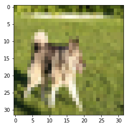
We can visualize a single random training example to see what the data looks like:
image_num = np.random.randint(0, network.size(train_data))
image_array = train_data[0][image_num].eval()
image_3d = image_array.reshape(3,32,32).transpose(1,2,0)

imshow(image_3d)
We’ll be using Michael Nielsen’s module which contains classes for different layer types. His classes handle things like weight initialization, passing parameters to/from other layers in the model, and simplifies the process of constructing a network. For example, the combined convolution and pooling layer (which we’ll be using) looks like this:
class ConvPoolLayer(object):
    """Used to create a combination of a convolutional and a max-pooling
    layer.  A more sophisticated implementation would separate the
    two, but for our purposes we'll always use them together, and it
    simplifies the code, so it makes sense to combine them.

    """

    def __init__(self, filter_shape, image_shape, border_mode='half',
                 stride=(1, 1), poolsize=(2, 2), activation_fn=sigmoid):
        """`filter_shape` is a tuple of length 4, whose entries are the number
        of filters, the number of input feature maps, the filter height, and
        the filter width.

        `image_shape` is a tuple of length 4, whose entries are the
        mini-batch size, the number of input feature maps, the image
        height, and the image width.

        `poolsize` is a tuple of length 2, whose entries are the y and
        x pooling sizes.

        """
        self.filter_shape = filter_shape
        self.image_shape = image_shape
        self.border_mode = border_mode
        self.stride = stride
        self.poolsize = poolsize
        self.activation_fn = activation_fn

        # initialize weights and biases
        n_in = np.prod(filter_shape[1:])  # Total number of input params
        # n_out = (filter_shape[0]*np.prod(filter_shape[2:])/np.prod(poolsize))
        self.w = theano.shared(
            np.asarray(
                np.random.normal(loc=0, scale=np.sqrt(1.0/n_in), size=filter_shape),
                dtype=theano.config.floatX),
            borrow=True)
        self.b = theano.shared(
            np.asarray(
                np.random.normal(loc=0, scale=1.0, size=(filter_shape[0],)),
                dtype=theano.config.floatX),
            borrow=True)
        self.params = [self.w, self.b]

    def set_inpt(self, inpt, inpt_dropout, mini_batch_size):
        # Reshape the input to 2D
        self.inpt = inpt.reshape(self.image_shape)

        # Do convolution
        self.conv_out = conv2d(
            input=self.inpt, filters=self.w, filter_shape=self.filter_shape,
            input_shape=self.image_shape, border_mode=self.border_mode,
            subsample=self.stride)

        # Get the feature maps for this layer
        self.feature_maps = theano.function([self.inpt], self.conv_out)

        # Max pooling
        pooled_out = pool.pool_2d(input=self.conv_out, ds=self.poolsize,
                                  ignore_border=True, mode='max')

        # Apply bias and activation and set as output
        self.output = self.activation_fn(
            pooled_out + self.b.dimshuffle('x', 0, 'x', 'x'))
        self.output_dropout = self.output # no dropout in convolutional layers

    def plot_filters(self, x, y, title, cmap=cm.gray):
        """Plot the filters after the (convolutional) layer.

        They are plotted in x by y format.  So, for example, if we
        have 20 filters in the layer, then we can call
        plot_filters(4, 5, "title") to get a 4 by 5 plot of all layer filters.
        """
        filters = self.w.eval()  # Get filter values/weights

        fig = plt.figure()
        fig.suptitle(title)

        for j in range(len(filters)):
            ax = fig.add_subplot(x, y, j+1)
            ax.matshow(filters[j][0], cmap=cmap)
            plt.xticks(np.array([]))
            plt.yticks(np.array([]))

        plt.tight_layout()
        fig.subplots_adjust(top=0.90)
        plt.show()
First we should set our mini-batch size, which is the number of training examples per batch. I use a small number here just for demonstration purposes, but how large of a batch size you use depends on how much memory you have available (this is mostly a concern if you’re training on a GPU with limited memory):
mini_batch_size = 10
Next, we define the network architecture by combining layers, setting their parameters, and choosing a minimization method (Stochastic Gradient Descent in this case). This method also allows you to train multiple networks for ensemble training by setting the value of the n parameter of the function:
def basic_conv(n=3, epochs=60):
    nets = []  # list of networks (for ensemble, if desired)
    for j in range(n):
        net = Network([
            ConvPoolLayer(image_shape=(mini_batch_size, 3, 32, 32),
                          filter_shape=(32, 3, 3, 3), stride=(1, 1),
                          poolsize=(2, 2), activation_fn=relu),
            ConvPoolLayer(image_shape=(mini_batch_size, 32, 16, 16),
                          filter_shape=(80, 32, 3, 3), stride=(1, 1),
                          poolsize=(2, 2), activation_fn=relu),
            ConvPoolLayer(image_shape=(mini_batch_size, 80, 8, 8),
                          filter_shape=(128, 80, 3, 3), stride=(1, 1),
                          poolsize=(2, 2), activation_fn=relu),
            FullyConnectedLayer(n_in=128*4*4, n_out=100),
            SoftmaxLayer(n_in=100, n_out=10)], mini_batch_size)

        net.SGD(train_data, epochs, mini_batch_size, 0.01,
                validation_data, test_data)

        nets.append(net)  # Add current network to list
    return nets
Finally, call the function to start training. Here I only train 1 network and only 10 epochs – ideally you’d want to train over many more epochs to obtain better model accuracy:
conv_net = basic_conv(n=1, epochs=10)
Results
During training, you can see the current epoch’s train/validation/test accuracy:
Training mini-batch 0/50000 | Cost: 2.3026 | Elapsed time: 0.02s
Training mini-batch 1000/50000 | Cost: 2.2458 | Elapsed time: 13.37s
Training mini-batch 2000/50000 | Cost: 2.3325 | Elapsed time: 26.95s
Training mini-batch 3000/50000 | Cost: 2.0104 | Elapsed time: 41.12s
Training mini-batch 4000/50000 | Cost: 1.8875 | Elapsed time: 54.77s
Epoch 0: Training accuracy 29.45%
Epoch 0: validation accuracy 30.40%
This is the best validation accuracy to date.
The corresponding test accuracy is 30.20%
Training mini-batch 5000/50000 | Cost: 1.7399 | Elapsed time: 100.68s
Training mini-batch 6000/50000 | Cost: 1.9128 | Elapsed time: 114.99s
Training mini-batch 7000/50000 | Cost: 2.1130 | Elapsed time: 128.68s
Training mini-batch 8000/50000 | Cost: 1.7989 | Elapsed time: 142.57s
Training mini-batch 9000/50000 | Cost: 1.5356 | Elapsed time: 156.34s
Epoch 1: Training accuracy 43.89%
Epoch 1: validation accuracy 44.12%
This is the best validation accuracy to date.
The corresponding test accuracy is 44.67%
Training mini-batch 10000/50000 | Cost: 1.2096 | Elapsed time: 199.59s
Training mini-batch 11000/50000 | Cost: 1.3554 | Elapsed time: 213.26s
Training mini-batch 12000/50000 | Cost: 2.0185 | Elapsed time: 226.95s
Training mini-batch 13000/50000 | Cost: 1.8238 | Elapsed time: 241.07s
Training mini-batch 14000/50000 | Cost: 1.3605 | Elapsed time: 254.85s
Epoch 2: Training accuracy 49.88%
Epoch 2: validation accuracy 49.86%
This is the best validation accuracy to date.
The corresponding test accuracy is 50.18%
Training mini-batch 15000/50000 | Cost: 1.1709 | Elapsed time: 296.85s
Training mini-batch 16000/50000 | Cost: 0.9121 | Elapsed time: 310.06s
Training mini-batch 17000/50000 | Cost: 1.7054 | Elapsed time: 323.39s
Training mini-batch 18000/50000 | Cost: 1.7038 | Elapsed time: 336.85s
Training mini-batch 19000/50000 | Cost: 1.2549 | Elapsed time: 350.36s
Epoch 3: Training accuracy 54.79%
Epoch 3: validation accuracy 54.20%
This is the best validation accuracy to date.
The corresponding test accuracy is 54.41%
Training mini-batch 20000/50000 | Cost: 1.1203 | Elapsed time: 392.55s
Training mini-batch 21000/50000 | Cost: 0.5949 | Elapsed time: 405.67s
Training mini-batch 22000/50000 | Cost: 1.5215 | Elapsed time: 419.14s
Training mini-batch 23000/50000 | Cost: 1.5645 | Elapsed time: 432.82s
Training mini-batch 24000/50000 | Cost: 1.1659 | Elapsed time: 447.61s
Epoch 4: Training accuracy 59.05%
Epoch 4: validation accuracy 58.09%
This is the best validation accuracy to date.
The corresponding test accuracy is 58.03%
Training mini-batch 25000/50000 | Cost: 0.9510 | Elapsed time: 491.26s
Training mini-batch 26000/50000 | Cost: 0.4127 | Elapsed time: 505.15s
Training mini-batch 27000/50000 | Cost: 1.3320 | Elapsed time: 519.11s
Training mini-batch 28000/50000 | Cost: 1.4922 | Elapsed time: 532.81s
Training mini-batch 29000/50000 | Cost: 0.9648 | Elapsed time: 546.87s
Epoch 5: Training accuracy 62.62%
Epoch 5: validation accuracy 60.40%
This is the best validation accuracy to date.
The corresponding test accuracy is 61.03%
Training mini-batch 30000/50000 | Cost: 0.7895 | Elapsed time: 590.57s
Training mini-batch 31000/50000 | Cost: 0.2871 | Elapsed time: 605.00s
Training mini-batch 32000/50000 | Cost: 1.2077 | Elapsed time: 619.68s
Training mini-batch 33000/50000 | Cost: 1.3634 | Elapsed time: 634.40s
Training mini-batch 34000/50000 | Cost: 0.7939 | Elapsed time: 650.52s
Epoch 6: Training accuracy 65.77%
Epoch 6: validation accuracy 62.45%
This is the best validation accuracy to date.
The corresponding test accuracy is 63.30%
Training mini-batch 35000/50000 | Cost: 0.6798 | Elapsed time: 693.56s
Training mini-batch 36000/50000 | Cost: 0.2129 | Elapsed time: 707.37s
Training mini-batch 37000/50000 | Cost: 1.1381 | Elapsed time: 721.11s
Training mini-batch 38000/50000 | Cost: 1.2876 | Elapsed time: 735.01s
Training mini-batch 39000/50000 | Cost: 0.6502 | Elapsed time: 748.82s
Epoch 7: Training accuracy 68.66%
Epoch 7: validation accuracy 64.50%
This is the best validation accuracy to date.
The corresponding test accuracy is 64.65%
Training mini-batch 40000/50000 | Cost: 0.6330 | Elapsed time: 791.59s
Training mini-batch 41000/50000 | Cost: 0.1772 | Elapsed time: 805.59s
Training mini-batch 42000/50000 | Cost: 0.9831 | Elapsed time: 819.47s
Training mini-batch 43000/50000 | Cost: 1.1417 | Elapsed time: 833.44s
Training mini-batch 44000/50000 | Cost: 0.5395 | Elapsed time: 847.47s
Epoch 8: Training accuracy 70.94%
Epoch 8: validation accuracy 66.00%
This is the best validation accuracy to date.
The corresponding test accuracy is 65.90%
Training mini-batch 45000/50000 | Cost: 0.5828 | Elapsed time: 889.95s
Training mini-batch 46000/50000 | Cost: 0.1658 | Elapsed time: 903.79s
Training mini-batch 47000/50000 | Cost: 0.8177 | Elapsed time: 917.53s
Training mini-batch 48000/50000 | Cost: 1.0552 | Elapsed time: 931.23s
Training mini-batch 49000/50000 | Cost: 0.4448 | Elapsed time: 944.75s
Epoch 9: Training accuracy 73.09%
Epoch 9: validation accuracy 67.21%
This is the best validation accuracy to date.
The corresponding test accuracy is 66.86%
Finished training network.
Best validation accuracy of 67.21% obtained at iteration 49999
Corresponding test accuracy of 66.86%
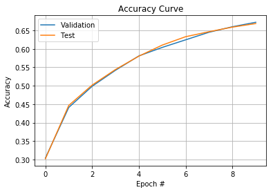
We achieved 66.86% test set accuracy after only 15 minutes of training over 10 epochs. There are many tweaks we could perform to improve accuracy, for example, changing the architecture of our model, or simply increasing the number of training epochs.
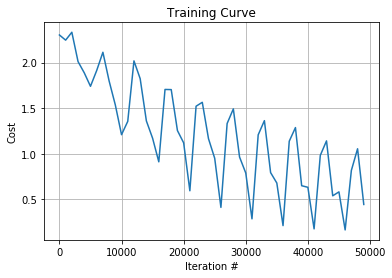
Finally, we can plot the training and accuracy curves to see how our model performed over time:
conv_net[0].plot_training_curve()
conv_net[0].plot_accuracy_curve()
Training a CNN for color image classification is very similar to training for grey scale classification. Additionally, using a package to handle the layers and passing of parameters (whether that’d be Lasagne, or a custom module like we used here) makes the process a whole lot easier.