XOR Logic Gate – Neural Networks
Introduction to neural networks and how they can be used to model XOR gates
February 13, 2017
Table of Contents
We have previously discussed OR logic gates and the importance of bias units in AND gates. Here, we will introduce the XOR gate and show why logistic regression can’t model the non-linearity required for this particular problem.
As always, the full code for these examples can be found in my GitHub repository here.
XOR gates output True if either of the inputs are True, but not both. It acts like a more specific version of the OR gate:
| Input 1 | Input 2 | Output |
|---|---|---|
| 0 | 0 | 0 |
| 0 | 1 | 1 |
| 1 | 0 | 1 |
| 1 | 1 | 0 |
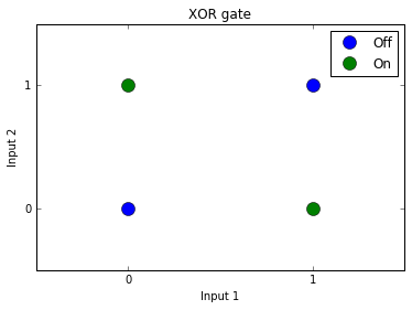
If we visualize the data space we’ll have a clearer sense of what causes the issue. As you can see, there is no linear separator that can effectively split the categories:
Logistic Regression
When we try to model this using logistic regression like the previous gate examples, we run into a problem:
import numpy as np
import theano
import theano.tensor as T

# Set inputs and correct output values
inputs = [[0,0], [1,1], [0,1], [1,0]]
outputs = [0, 0, 1, 1]

# Set training parameters
alpha = 0.1 # Learning rate
training_iterations = 30000

# Define tensors
x = T.matrix("x")
y = T.vector("y")
b = theano.shared(value=1.0, name='b')

# Set random seed
rng = np.random.RandomState(2345)

# Initialize random weights
w_values = np.asarray(rng.uniform(low=-1, high=1, size=(2, 1)),
                      dtype=theano.config.floatX) # Force type to 32bit float for GPU
w = theano.shared(value=w_values, name='w', borrow=True)

# Theano symbolic expressions
hypothesis = T.nnet.sigmoid(T.dot(x, w) + b) # Sigmoid/logistic activation
hypothesis = T.flatten(hypothesis) # This needs to be flattened so
                                   # hypothesis (matrix) and
                                   # y (vector) have the same shape

cost = T.nnet.binary_crossentropy(hypothesis, y).mean() # Binary CE
updates_rules = [
    (w, w - alpha * T.grad(cost, wrt=w)),
    (b, b - alpha * T.grad(cost, wrt=b))
]

# Theano compiled functions
train = theano.function(inputs=[x, y], outputs=[hypothesis, cost],
                        updates=updates_rules)
predict = theano.function(inputs=[x], outputs=[hypothesis])

# Training
cost_history = []

for i in range(training_iterations):
    h, cost = train(inputs, outputs)
    cost_history.append(cost)
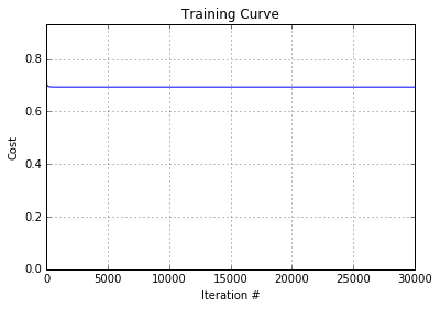
The network is unable to learn the correct weights due to the solution being non-linear. We can see this by looking at the training curve:
Introducing neural networks
One way to solve this problem is by adding non-linearity to the model with a hidden layer, thus turning this into a neural network model.
As always, we begin with imports and defining the data and corresponding labels:
import numpy as np
import theano
import theano.tensor as T

# Set inputs and correct output values
inputs = [[0,0], [1,1], [0,1], [1,0]]
outputs = [0, 0, 1, 1]
Next, we define some training parameters. hidden_layer_nodes is used to control the number of units/neurons in the hidden layer. This will be useful when we set up the network architecture later:
alpha = 0.1 # Learning rate
training_iterations = 50000
hidden_layer_nodes = 3
Then, define our tensors and weight arrays. Note the inclusion of b2 which is the bias for our hidden layer neurons and a second array of weights (w2_array) for the hidden layer to output layer connections.
# Define tensors
x = T.matrix("x")
y = T.vector("y")
b1 = theano.shared(value=1.0, name='b1')
b2 = theano.shared(value=1.0, name='b2')

# Set random seed
rng = np.random.RandomState(2345)

# Initialize weights
w1_array = np.asarray(rng.uniform(low=-1, high=1, size=(2, hidden_layer_nodes)),
                      dtype=theano.config.floatX) # Force type to 32bit float for GPU
w1 = theano.shared(value=w1_array, name='w1', borrow=True)

w2_array = np.asarray(rng.uniform(low=-1, high=1, size=(hidden_layer_nodes, 1)),
                      dtype=theano.config.floatX) # Force type to 32bit float for GPU
w2 = theano.shared(value=w2_array, name='w2', borrow=True)
We need some additional expressions to evaluate the output values of both the input (a1) and hidden (a2) layers:
a1 = T.nnet.sigmoid(T.dot(x, w1) + b1)  # Input -> Hidden
a2 = T.nnet.sigmoid(T.dot(a1, w2) + b2) # Hidden -> Output
hypothesis = T.flatten(a2) # This needs to be flattened so
                           # hypothesis (matrix) and
                           # y (vector) have the same shape

cost = T.nnet.binary_crossentropy(hypothesis, y).mean() # Binary CE
Remember to add update rules for the additional weights (w2) and biases (b2) that we added:
updates_rules = [
    (w1, w1 - alpha * T.grad(cost, wrt=w1)),
    (w2, w2 - alpha * T.grad(cost, wrt=w2)),
    (b1, b1 - alpha * T.grad(cost, wrt=b1)),
    (b2, b2 - alpha * T.grad(cost, wrt=b2))
]
We finish off with some Theano functions and the actual training process:
train = theano.function(inputs=[x, y], outputs=[hypothesis, cost],
                        updates=updates_rules)
predict = theano.function(inputs=[x], outputs=[hypothesis])

# Training
cost_history = []

for i in range(training_iterations):
    h, cost = train(inputs, outputs)
    cost_history.append(cost)
The full code can be found here.
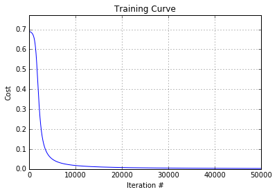
After training this neural network we can see that the cost correctly decreases over training iterations and outputs our correct predictions for the XOR gate: